Elo Scores and Squash Ratings: The Art of Quantifying Skill

As squash enthusiasts, we tend to be quite analytical, always seeking new ways to think about our beloved sport. Today, I want to delve into the fascinating world of Elo scores and squash ratings, exploring how these metrics help us understand and quantify player skill levels.

The Elo Rating System: From Chess to Squash

Elo scores are most well-known from chess, with ratings ranging from below 1000 to over 2700. Chess Grandmasters, who must have ratings between 2500-2700 to earn the title, are recognized worldwide for their exceptional skill. Interestingly, as of 2024, 42 women have been awarded the GM title out of about 2000 Grandmasters.

But enough about chess—let’s talk squash! Elo scores can be adapted to any context comparing the relative skill levels of players, making them perfect for head-to-head squash matches. The Club Locker or Universal Squash Rating (USR) system used in the US goes from 1.0 (beginners) to beyond 7.0 for pros. Although initially based on Elo scores, the current system, redesigned by Elder Research between 2012-2014, has evolved to increase predictive accuracy. The new system, which weights recent games more heavily, gained a 10% increase in accuracy upon release.

The Unique Dynamics of Squash Ratings

The USR system differs from pure Elo ratings by incorporating a recency weighting and reliability score. It considers only matches played within the last 45 months, emphasizing the most recent 15 months. This ensures that current form and skill levels are more accurately reflected in the ratings.

US Squash recommends competing with players within ±0.5 of your rating. Matches with a greater differential are often disregarded if the higher-rated player wins, as they provide little insight into the higher-rated player’s skill. An analysis of ~80,000 matches found that for each 0.1 rating gap, the probability of the higher-rated player winning increases by 15%, but only if the ratings are within 0.25 of each other. Beyond a 0.5 differential, the outcome becomes a foregone conclusion.

The current state of women’s squash

To put these ratings into perspective, let’s look at the current world number one women’s squash player, Nour El Sherbini. She’s an absolute powerhouse on the court, and her impressive rating reflects her dominance in the sport. This rating means that any match between El Sherbini and me would inevitably result in a series of straight losses for me — I’d be collecting straight losses faster than I can say “game, set, match!”

Nour El Sherbini after defeating Nouran Gohar:

Her rating:

Understanding and Simulating Elo Ratings in Squash

To better grasp how these ratings work, let’s build our own Elo system and simulate some squash matches. We’ll first go through some notation to understand how skill factors into the probability of a player winning.

Calculate the probability of Player A winning

The probability that A defeats B given their respective skill levels (with \(k\) as a scaling factor):

\(P(\text{A defeats B}|\theta_A, \theta_B) = \frac{1}{1+e^{(-k(\theta_A-\theta_B)}}\)

To illustrate this, let’s simulate some squash matches.

From now on, I will use \(\theta\) and ability level interchangeably.

library(tidyverse)
library(kableExtra)

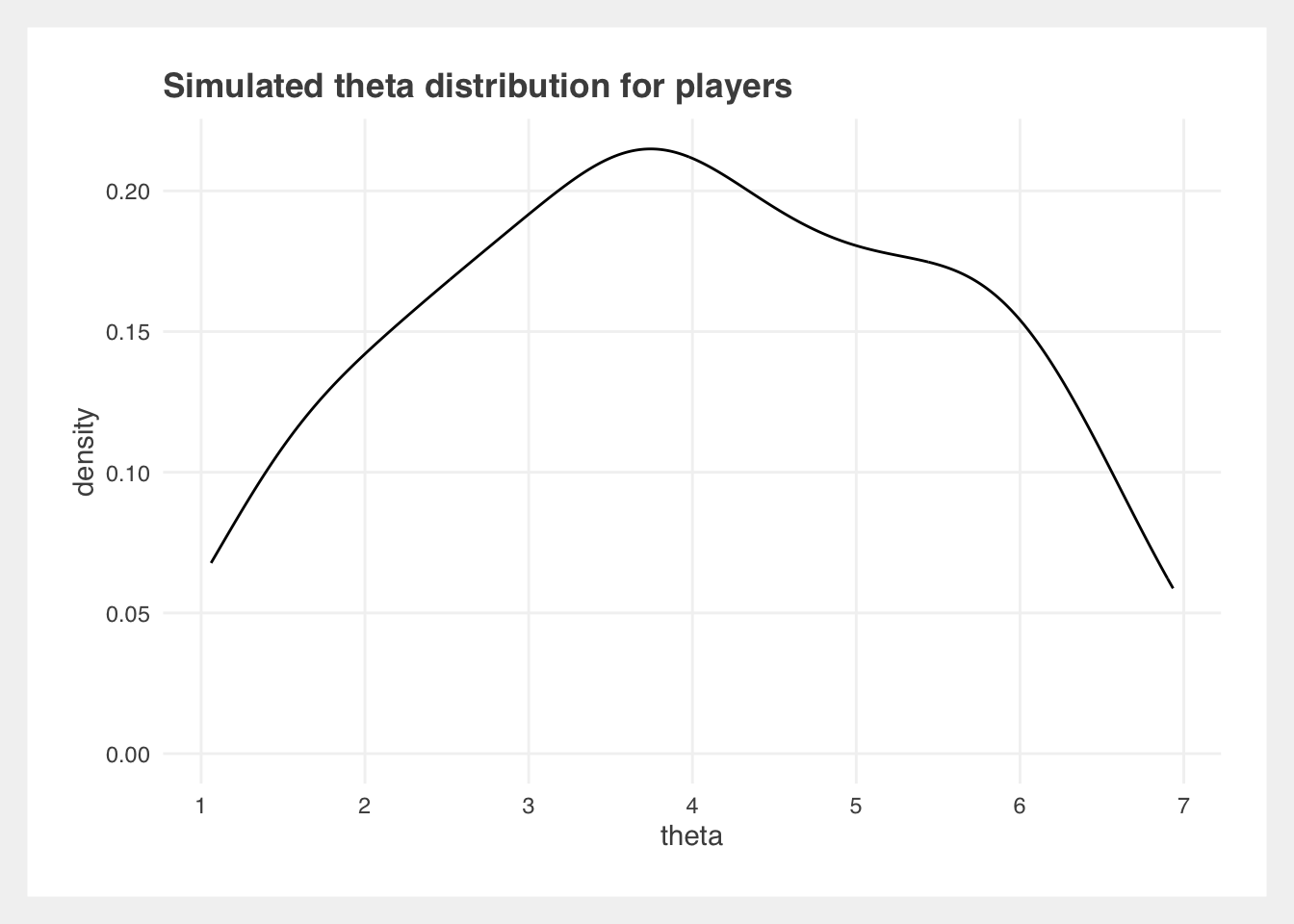
Simulate data for 100 players, and give them each a true ability level, which will be used later to calculate the probability of winning a match.

players <- data.frame(
  id = 1:100,
  # set up a bounded normal distribution, bound between 1 and 7
  theta = qnorm(p = runif(
    n = 100,
    min = pnorm(1, 3.5, 2),
    max = pnorm(7, 3.5, 2)
  ), mean = 3.5, sd = 2)
)

players |>
  arrange(-theta) |>
  slice(1:6) |>
  ggplot(aes(y = theta, x = reorder(id, -theta))) +
  geom_bar(stat = "identity", fill = "lightblue") +
  geom_text(aes(label = round(theta, 2)), vjust = 1.8) +
  labs(x = "Player ID", y = "theta", title = "Top 6 players by theta")

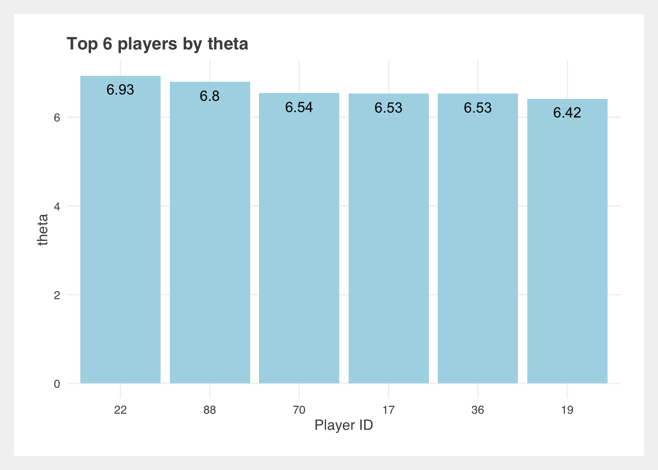
Take note of the best players: 22 and 88.

Next, we simulate outcomes of 1000 matches. Using the equation above, we can give rbinom the probability that Player A wins the match, given the \(\theta\) of both Player A and Player B.

ids <- 1:100
matches <- data.frame(
  player_1 = sample(x = ids, size = 1000, replace = T),
  player_2 = sample(x = ids, size = 1000, replace = T)
) |>
  filter(player_1 != player_2) |>
  rowwise() |>
  # k was set at 1
  mutate(result = rbinom(n = 1, size = 1, prob = 1 / (1 + exp(-1 * (players[player_1, "theta"] - players[player_2, "theta"])))))

Just to confirm that players with higher ability levels should be winning more of their matches, we calculate the win rate. Since the original matches dataframe has one row per match, with result being 1 if Player 1 won, matches_full duplicates each match and flips the player IDs so that we can calculate their win rate across all matches.

matches_flipped <- matches |>
  mutate(
    player_1_new = player_2,
    player_2 = player_1,
    result = 1 - result
  ) |>
  select(-player_1) |>
  rename(player_1 = player_1_new) |>
  select(player_1, player_2, result)
matches_full <- matches |> bind_rows(matches_flipped)
ranked_players <- matches_full |>
  group_by(player_1) |>
  summarise(win_rate = mean(result)) |>
  arrange(-win_rate)

win_rates <- inner_join(ranked_players, players, by = join_by(player_1 == id)) |>
  arrange(-win_rate)

head(win_rates) |>
  kable(col.names = c("Player", "Win Rate", "Theta"), caption = "Top 6 players", digits = 2) |>
  kable_styling(position = "center", full_width = F)

As expected, the top few players have the highest win rates!

ggplot(win_rates, aes(x = theta, y = win_rate)) +
  geom_point() +
  labs(y = "win rate", title = "Win rate by theta")

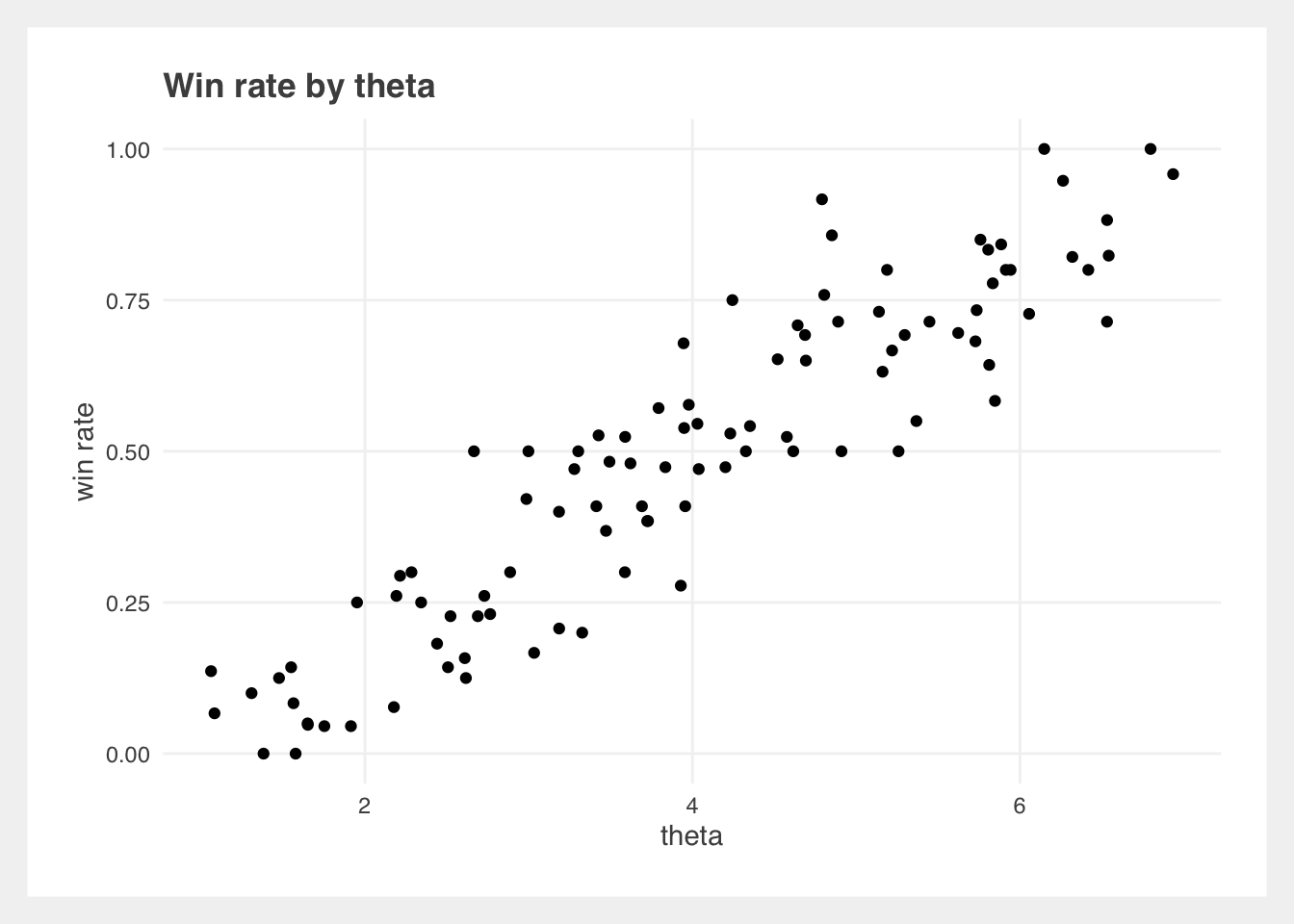
The Win rate by theta plot shows us that win rate increases with theta, which is what we expect. However, there is some randomness in the plot! Ratings will never perfectly predict results. A higher rated player does not always beat a lower rated player, although we can expect a predictable outcome if there is a large enough difference in ratings, and enough matches are played (the central limit theorem at work!).

Use optim to estimate player’s ability levels

In reality, we don’t know the true ability levels of players — we only have match outcomes. However, because we simulated their true ability levels, we can see how well this worked in estimating that.

The built-in optim function in R is used to find the minimum or maximum of a function. In this case, I maximise the log-likelihood to estimate the ability level of each player.

LogLikMatch <- function(data, theta) {
  p <- plogis(theta[data$player_1] - theta[data$player_2])
  ll <- sum(data$result * log(p) + (1 - data$result) * log(1 - p))
  return(ll)
}
starting_theta <- rep(0.5, 100)

solution <- optim(starting_theta, LogLikMatch,
  data = matches,
  # this method generally works well for box-constrained optimization
  method = "L-BFGS-B",
  lower = 1, upper = 7,
  # fnscale will swap the minimum likelihood to make it maximum likelihood
  # also set maxit to allow for more iterations
  control = list(fnscale = -1, maxit = 1e6)
)

players <- players |> bind_cols(est_theta = solution$par)

ggplot(players, aes(x = theta, y = est_theta)) +
  geom_point() +
  geom_abline(intercept = 0, slope = 1, lty = "dotted") +
  labs(y = "estimated theta", title = "Estimated theta vs theta")

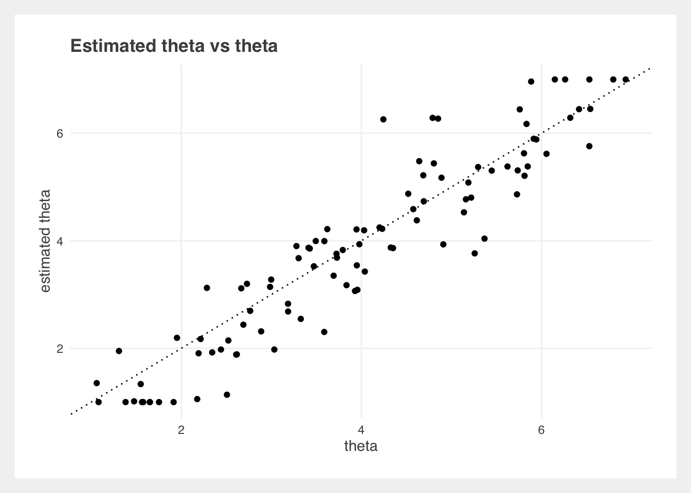
Compare estimated \(\theta\) with the real \(\theta\) we originally created:

As shown, our estimated ability levels are quite close to the true levels, demonstrating the effectiveness of our Elo-based simulation.

Note: The original simulated \(\theta\) distribution does not have a perfectly normal distribution, and the maximum likelihood estimator was bounded to 1 and 7, so the estimates are on a slightly different scale from the original.

range(players$theta)

## [1] 1.060522 6.934806

range(players$est_theta)

## [1] 1 7

The Takeaway

Understanding and applying Elo ratings to squash not only enriches our appreciation of the game but also offers valuable insights into player performance. By quantifying skill levels, we can make more informed decisions about competition and training. Whether you’re a player or a fan, these metrics add a new dimension to your squash experience.